Lupine Publishers: Lupine Publishers | The Prevention and Treatment o...

Lupine Publishers: Lupine Publishers | The Prevention and Treatment o...: Lupine Publishers | Open access Journal of Complimentary and Alternative Medicine Abstract Native people in West Timor In...

Lupine Publishers| Socioeconomic Variables Associated with Level of Obesity and Prevalence of Other Diseases Among Children and Adolescents of Some Affluent Families of Bangladesh

Lupine Publishers| Journal Of Diabetes and Obesity

Abstract

The present study utilized the data collected from 662 children observed from 560 randomly selected families of students of American International University-Bangladesh. Among the investigated children and adolescents 465 were in underweight group. Obesity and severe obesity were observed among 9.1 percent children and adolescents and prevalence of diabetes was observed among 22.8 percent respondents. The percentage of respondents affected by different diseases except diabetes was 13.4. It was evident that level of obesity, prevalence of diabetes and prevalence of other diseases were significantly associated, and level of obesity was associated with different socioeconomic characters of the parents and of the respondents. Parents’ education, age of children, family income and food habit of the children were the most important variables for the change in level of obesity of children and adolescents. Fitting of logistic regression using level of other diseases as dependent variable showed that residence, parents’ education, family income, prevalence of diabetes, food habit of the children, blood sugar level of children, utilization of time by the children were some of the variables responsible for prevalence of other diseases among the children.
Keywords:Level of obesity; Socioeconomic variables; Significant association between diabetes and level of obesity; Logistic regression

Introduction

Child overweight and obesity are the most serious public health challenges of the 21^st century worldwide , specially, in low and middle-income countries. It affects mostly the urban people [1,2]. The obesity for child and adolescents is measured by body mass index [BMI = weight in kg / (height in meter²] , where children having BMI above the 85^th percentile are considered as overweight and those who have BMI above the 95^th percentile are considered as obese [3]. The level of obesity is increasing at alarming rate. In a global study in 2016 it was estimated that over 41 million [1] children under the age 5 years were overweight. The prevalence of overweight in adolescents is defined by BMI + standard deviation of BMI and obesity for them is decided by BMI + 2 standard deviation [1]. Overweight and obesity are defined as abnormal or excessive fat accumulation that presents a risk to health. Child obesity can lead to life threating conditions including diabetes, heart disease, sleep problems, cancer, liver disease, early puberty, eating disorders, skin infection, asthma and other respiratory problems [4]. The adolescent’s obesity leads to the problem of hepatitis, sleep aponia, and increased intercranial pressure [5].
The other effects of overweight and obesity are psychological [6], depression [7], physical [8,9]. The early physical effect of obesity in adolescence is noted when it affects all most all the organ which leads to the increase rate of mortality in adulthood [4,10]. The causes of childhood obesity are genetic. Over 200 genes affect weight by determining activity level, food preferences, body type, and metabolism [4]. Family practices such as decreasing rate of breast feed, by mothers, stay home and utilizes electronic devices, less physical activity, food habit, specially, taking more calorie food from restaurant with less fiber [4,9,11], low socioeconomic status [12], eating habit of calorie- rich drinks [13]. However, the problem can be obviated by avoiding the sources of causes of obesity and encouraging the children and adolescents to be involved in physical activities. From the above discussion, it can be concluded that growing level of obesity among children and youth and increasing the rate of prevalence of diabetes are of great concern throughout the world. Many of the complications are silent and often go undiagnosed. The obese children are at high risk for the development of early morbidity. Considering all these aspects discussed above, the objective of the study was planned to observe the joint relationship of level of obesity and prevalence of diabetes including prevalence of other diseases with other socioeconomic factors which were more responsible for the variation in the level of obesity among children and adolescents under 18 years of age coming out from affluent families. The specific objective was to investigate the association of level of obesity of children and adolescents with some social factors. Also, to identify the responsible variable for other diseases.

Methodology

For the analysis it was decided to collect information from children of affluent families. In a separate [14,15] families of students of American International University - Bangladesh were identified as affluent families. Hence, it was planes to collect data from some randomly selected families of students of the abovementioned university. In a previous study [16] it was reported that there were 7% overweight and obese children and youth in Bangladesh. Accordingly, we had decided to have a proportion of at least 7% overweight and obese children and youth with margin of error of 2% at 95% confidence. Accordingly, for a simple random sample the sample the calculated value of sample size was an=625. This sample size covered 6.6% students of the university. The sample students were selected by simple random sampling method and were expecting at least responses from 5% families of the students. However, information was received from 560 families, covering the data of 662 children.
The data were collected through pre-designed and pre-tested printed questionnaire covering the questions related to the demographic characteristics of the children and adolescents of age below 18 years and the questions related to the socioeconomic variables of the parents. The randomly selected students were given written instructions how to collect information and they were requested to help in collecting information from their parents, who were very much concerned about the health hazard of their offspring. The parents of children filled in the questionnaires as some of the children were under 18 years of age and some were even below 10 years. The important collected information was age, height, weight, sex, food habit, time spent, involvement in co-curricular activities, if it is feasible, of the children, and information regarding the prevalence of any other diseases. To study the socioeconomic background of the children, the information regarding parent’s level of education, occupation and income were also collected. For youth having diabetes, the latest blood sugar level measured by registered practitioner or measured in a registered clinic also recorded. Association of level of obesity of offspring with families’ socioeconomic background were examined using chi-square test, where significant association was concluded when p-value ≤0.05. Logistic regression model using levels of prevalence of other diseases as dependent variable was fitted.

Result and Discussion

The present analysis was done using the data of social, medical and economic aspects of 662 children of age less than or equal to 18 years investigated from 560 randomly selected families of the students of American International University – Bangladesh. From the analysis it was noted that 22.8 percent children were affected by diabetes. This percentage among the obese and severe obese group of children was 32.2 indicating that level of obesity and prevalence of diabetes was significantly associated
[ χ2 =8.741, p-value = 0.033, Table 1]
Considering the prevalence of diabetes among the obese and severe obese group compared to non-obese group, the former group were 69 percent more exposed to the problem of diabetes [O.R = 1.69]. Their risk ratio was 1.47 compared to non-obese group. Amongst the investigated children 70.2 percent were in underweight group and 9.1 percent were in obese and severe obese group. The level of obesity was measured by the amount of BMI (weight in kg / height in m²). The mean value of BMI was 17.67 with a standard deviation 10.58. The underweight group of children and adolescents had BMI <23. The BMI of other three groups were 23 - <30, 30 - <45 and 45+. The levels of BMI were decided according to the percentile values. This finding was almost similar to that observed in another study [15]. Amongst the observed children and adolescent’s 78.1 percent were in the age group 10 years and above and 70.2 percent of the investigated children and youth were in underweight group and 9.1 percent were obese and severely obese. Majority [ Table 2, 78.2%] of them were in the age group 10 years and above and among them 72.6 percent were in underweight group. In these group obese and severe obese children were 6.9 percent. Major obese and severe obese children (19.4%) were among the children of age 5 to less than 10 years. The differences in the proportions of levels of obesity according to different age groups were significant [ χ2 = 39.043, p- value = 0.000]. The prevalence of obesity and severe obesity among the children of age group 5 to less than 10 years compared to children of other age groups were too high [O.R = 13.06]. Let us investigate the prevalence of diabetes and prevalence of other diseases among the children and adolescents. It was observed that 86.6 percent investigated children had no other health hazard (Table 2) except diabetes. However, 21.2 percent of them were diabetic patients. Among the diabetic patient’s 11.3 percent had eye problem. The major problem among the respondents was eye problem. The percentage of this group of children was 7.6. There were significant differences in the percentages of respondents facing health hazard according to prevalence of diabetes [χ2 = 10.957, p-value = 0.027].

Table 1: Distribution of respondents according to level of obesity and prevalence of diabetes.

Table 2: Distribution of children according to prevalence of diabetes and prevalence of other diseases.

Now, let us investigate the reason of obesity and severe obesity among the children and youth. Some of the social factors might have enhanced the level of obesity. This was noted from the study of association of different factors and level of obesity. The investigated children and adolescents were classified into three classes by their age levels. These three groups of children were again classified by their level of obesity. The classified results were shown in Table 3. It was seen that 72.5% children and youth of the age group 10 years and above were underweight. The proportions of underweight children of other two age groups were lesser than the percentages of overall underweight group of children. The children less than 5 years of age had the highest percentage of the overweight group and this group of children had the 58 percent [O.R.=1.58] more chance of overweight compared to other groups of children. This differential in proportions of level of obesity according to age groups was highly significant [ χ2 = 38.94, p-value=0.000]. Amongst the studied children 58.2 percent were males (Table 4) and 77.4 percent of them were underweight. The corresponding figure among females is 60.3 percent. The differential in obesity by sex differences is significant [ χ2= 44.03, p-value= 0.00]. Number of children of different levels of obesity belonging to different residential areas were presented in (Table 5). It was seen that maximum village children (76.5%) were underweight compared to urban semiurban children. Again, among the village children, number of obese and severe obese groups were lower compared to other groups of children. The differences in proportion. The information of 72.5% children were reported from urban area. The corresponding percentages of rural and semi-urban children were 18 and 9.5. The classified information of level of obesity and residence of children were significantly different [ χ2 = 12.45, p-value= 0.04]. Similar findings were observed in other studies [14,15] It was already mentioned that the study group of children were mostly living in city center (72.5%) and though they had the enough scope to be involved in physical activities like games and sports, still majority of the children (39.9%) passed their time by watching television and 16.8% slept after or before their academic activities. One-fourth (26.4%) of the investigated children mentioned that they were involved in some other activities including games and sports (Table 6). Around 72% severe obese group killed their time by watching television. The corresponding percentage among obese group is 45.2. The differentials in proportions of utilization of time by the children of different obese groups were significantly different as [χ2= 54.12 with p- value = 0.00]. Let us now observe the food habit of investigated children and adolescent. As the investigating units were mostly from affluent city residence, they had the scope to get sufficient foods, with proper hygienic measures. Among the investigating units’ 47.9 percent were habituated in taking food from restaurants. Among the obese children 54.7 percent were habituated in takin restaurant food (Table 7).

Table 3: Distribution of children and adolescents according to their age and level of obesity.

Table 4: Distribution of children according to their gender and level of obesity.

Table 5: Distribution of children according to their residence and level of obesity.

Table 6: Distribution of children according to their utilization of time and level of obesity.

Table 7: Distribution of children and adolescents according to their food habit and level of Obesity.

In a separate study [15] it was reported that the increasing trend of obesity was associated with fast food from restaurant. Of course, higher proportions of underweight (46.9%) and overweight group of children (53.3%) were habituated in taking restaurant food. However, the differentials in proportions of children taking restaurant food according to different levels of obesity were significant [ χ2 = 94.63 with p-value = 0.00]. Usually the children of affluent families were more likely to be stay back in the house and kill time by watching television. These children also had more chances to frequently visit fast food shops. Their parents could afford the cost of fast foods and they were also fulfilled the demand of their children if they had sufficient family income. It was observed that the monthly family income of 38.2% families was 70 thousand and above taka [ Bangladesh currency] but 79.1 % children of these families were in underweight group (Table 8). It was seen that prevalence of obesity was higher among the children of low-income group of families. This differential in observing obesity was significantly different among the low-income group of families [ χ2 = 53.06 with p-value = 0.00]. Family environment was one of the correlates of obesity among children [16]. It seemed that family environment was influenced by parents’ education and occupation. Let us investigate how fathers’ and mothers’ education were associated with children and adolescent’s obesity. It was seen that (Table 9) the fathers of 77.9 % children were higher educated and 75% children of them were underweight. The percentage of illiterate fathers was 3.5 and 91% children of these fathers were underweight. But obesity and severe obesity among children of illiterate and primary educated fathers were more (8.7 and 17.4% respectively) compared to the children of secondary educated (2.1%) fathers. The differential in proportions of level of obesity and fathers’ educational level were highly significant [χ2 = 111.70 with p-value = 0.00]. Similar significant differentials in proportions of obesity of children according to the differences of mothers’ education were also observed [Table 10 χ2 = 39.23 with p-value = 0.00].

Table 8: Distribution of children and adolescents according to their level of obesity and monthly Income.

Table 9: Distribution of children and adolescents according to their level of obesity and level of father’s education.

Table 10: Distribution of children and adolescents according to their level of obesity and level of mother’s education.

There were 5.1 percent agriculturists and 79.4 percent children of them were underweight. The lowest underweight children were observed in those families where father was engaged in profession other that business and service. The maximum underweight children were observed in the families where father was a serviceman. The differential in proportions in different levels of obesity by father’s occupation was significant [χ2 =67.281, p-value=0.000, Table 11]. However, mothers occupation had no impact on level of obesity of children and adolescents [ χ2 =6.279, p-value=0.393, Table 12].

Table 11: Distribution of children and adolescents according to their level of obesity and levels of father’s occupation.

Table 12: Distribution of children according to their level of obesity and level of mother’s occupation.

Association between level of obesity and some social characters were studied by chi-square test. Here impact of social variables on obesity and prevalence of diabetes were not studied. It was done in some other study [19]. However, the impacts of social factors on prevalence of other diseases were studied. It was done by fitting the logistic regression model assuming levels of other diseases as dependent variable. The explanatory variables used were residence, religion, age, parent’s education, parent’s occupation, family income, food habit of children, utilization of time by the children, blood sugar level of them and body mass index. However, all the variables were not used in fitting the final model because during observing model fitting criteria some variables were found insignificant. These variables were age of children, gender of children and parents’ occupation. The analytical results were shown below: From the fitted model it was noticed that prevalence of diabetes, level of obesity, and residence were the responsible factors for the prevalence of other diseases. The analysis was done considering no disease as reference factor Table 13. Thus, Model fitted results were available for the remaining 4 types of diseases. However, due to insignificant results in fitting the model for the diseases like kidney problem, hypertension and some other diseases the results were not presented. Results were presented only for the disease eye problem. This problem was prevailed among 7.6 percent respondents and this group was the biggest (56.2 %) among the children and adolescents who were experienced of different diseases. The fitted model was significant as was observed by the statistic – 2loglikelihood =364.489 and the corresponding χ2 = 1696.824 with p-value =0.000. The value of Cox and Snell R²=0.923 and Nagelkerke R²= 0.961.

Conclusion

The present study was conducted to observe the level of obesity, prevalence of diabetes and prevalence of other diseases among children and adolescents of some randomly selected families of the students of American International University-Bangladesh. Most of the families were city dwellers and these families were socially and economically in better position [17-19] compared to the general people of Bangladesh. However, the obesity and severe obesity among children were similar to that of the general people of the country. Obesity and severe obesity were associated with the parent’s social and economic status. Occupation, family income and age of children and youth were the most important factors to influence the level of obesity. The study indicated that prevalence of diabetes was dependent on level of obesity and both these characteristics were the problem for both parents and health planners. Parents can take care of foods of their offspring and motivate to take home foods as per as possible avoiding the restaurant foods Table 14. They can motivate their kids to spend their time in doing some activities related to physical work in addition to their academic works. Logistic regression model was fitted to identify the responsible variable for the prevalence of other diseases. It was observed that family income, prevalence of diabetes and level of obesity were some of the responsible variables for the diseases.

Table 13: Model fitting criteria.

Table 14: Results Related to Fitted Logistic Regression Model.

Problems of obesity are manifold. It is a life threating condition which can enhance diabetes, heart disease, cancer, liver disease, skin infection, asthma, and other respiratory problems [20,21]. Obese adolescents have increased chance of mortality during adulthood [22]. The problem also arises from the social environment. Hence, some measures need to be taken to control the problem. Government and school authority should introduce some regulations so that physical education is a compulsory cocurricular activity of the school. Parents can encourage their kids to avoid watching television and untimely sleeping and they can provide the quality school lunches. Kids should be provided fresh and healthy food and they should be accompanied to parks and to play field or walkways. They can be advised to avoid sedentary activities like use of mobile phone, computer, video games. Some of the steps of parents can prevent the alarming increase in the rates of obesity and severe obesity and in the rate of prevalence of diabetes and prevalence of other diseases.

For more Lupine Publishers Open Access Journals Please visit our website:
http://lupinepublishers.us/

For more Open Access Journal on diabetes and Obesity articles Please Click Here:
https://lupinepublishers.com/diabetes-obesity-journal/

To Know More About Open Access Publishers Please Click on Lupine Publishers

Follow on Linkedin : https://www.linkedin.com/company/lupinepublishers

Follow on Twitter   :  https://twitter.com/lupine_online

Lupine Publishers: Lupine Publishers | Acute Erythroblastic Leukemia ...

Lupine Publishers: Lupine Publishers | Acute Erythroblastic Leukemia ...: Lupine Publishers | Open Access Journal of Oncology and Medicine   Abstract Acute erythroblastic leukemia is characteriz...

Lupine Publishers: Lupine Publishers | Principles of the Military Con...

Lupine Publishers: Lupine Publishers | Principles of the Military Con...: Lupine Publishers- Anthropological and Archaeological Sciences Journal Impact Factor   Introduction A way from the regular th...

Lupine Publishers: Lupine Publishers | Principles of the Military Con...

Lupine Publishers: Lupine Publishers | Principles of the Military Con...: Lupine Publishers- Anthropological and Archaeological Sciences Journal Impact Factor   Introduction A way from the regular th...

Lupine Publishers: Lupine Publishers | Peer Review of Statistics in S...

Lupine Publishers: Lupine Publishers | Peer Review of Statistics in S...: Lupine Publishers | Journal of Cardiology & Clinical Research     Opinion Professor Peter Bacchetti’s excelle...

Lupine Publishers| A Note on the Application of Discriminant Analysis in Medical Research

Diabetes and Obesity Open access Journals- Lupine Publishers

Introduction

The social aspects of medical research and research in life science deal with data collected from randomly selected investigating units either by direct interview or by doing some controlled experiments. The objective of investigation is to verify the existence of some pre-assumed hypothesis and belief. Whatever be the objective of the research, the study is done using the collected data, where the data are either categorical or numerical or both. There are many advanced statistical methods [1] to handle the data, especially if the data are numerical. Limited number of methods of analysis is there to handle the categorical data. But proper statistical methods are to be applied to study the unknown characteristics in the population. Once the technique of analysis is identified, the analysis can be done using any one of the Statistical Packages available for the analysis. The major source of data in the field of life science and medical science is related to public health and the main aspect of analysis is to suggest ways and means to improve the health status of the public by controlling the diseases which are fatal as well as causes of health hazard in the society. Any type of health hazard is the cause of economic and social problems for the country as well as for the family. Thus, the health planners need the proper analytical findings to formulate the guidelines so that the health hazard is reduced to a great extent. The data are collected from each and every investigating unit.
Some of the data are age, height, weight, level of education, occupation, income, marital status, type of work, food habit, smoking habit, prevalence of obesity, diabetes, hypertension, etc. The prevalence of obesity is the cause of non-communicable diseases like diabetes and hypertension and the sources of these two are occupation, work type, food habit, smoking habit. There may be other sources of diseases. But the sources mentioned here are categorical (qualitative) variable. The quantitative variable income, age, weight, etc. are also the sources of non-communicable diseases [2]. The data mentioned above are the multivariate data. The analytical procedures of these data are different, and the procedures are broadly classified as
a)Dependence Analysis
b)Interdependence Analysis.
One of the techniques of dependence analysis is the Discriminant Analysis. This analysis is used to discriminate the investigated units according to some categorical variable and to identify the most responsible variable(s) for the discrimination. Accordingly, the health planners can suggest the ways and means so that proper action can be taken to control the sources responsible for the health hazard in the society.
Discriminant Analysis
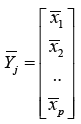
Let x_ij be the i-th variable observed from j-th category of units [ i = 1, 2, ……..p ; j= 1, 2, …., k], where

S_j = Variance- Covariance matrix of (x_{i j}) , S_u = Combined variance- covariance matrix, where
S_u = Σ n_j S_j / ( n – k ). Here n_j = number of observation in j- th category, n = Σ n_j.
The k category of units can be discriminated by
a)ML Method of Discrimination
b)Bayes Discriminant Rule and
c)Fisher’s Discriminant Rule.
The ML method of discrimination needs to calculate the following statistic

where j ≠ k.If we consider that k = 3, then there exists linear relationship of the type
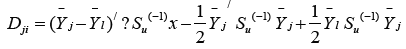
D₁₂ + D₂₃ = D₁₃.
In such a situation the value of x will be allocated to a population as per the rule discussed below:
a) If D₁₂>0 and D₁₃>0, allocate x to the population -1
b) If D₁₂<0 and D₁₃>0, allocate x to the population -2
c) If D₁₂<0 and D₁₃<0, allocate x to the population -3.
The discriminant analysis is meaningful if the k mean vectors of variables are heterogeneous. For the analysis a model is considered when there are k = 2 groups, where the model is
D = B₀ +B₁ x₁ + B₂ x₂ + …………. + B_p x_p
Here B_i (i = 1, 2, ….,p) is the discriminant coefficient of the variable xi . The interpretation of these coefficients are closely follows the logic of multiple regression. The value Bi indicates the importance of the variable xi in discriminating between the two groups. For k=3 groups problem, one function is considered to discriminate between first group and combined second and third group. Another function is considered to discriminate between second and third group. The number of discriminant functions are (k – 1) if their k groups. In that case the interpretation of coefficients is made for each function separately. The coefficients are available using Statistical Packages. D is the discriminant score for different values of x when k=2. The correlation coefficient of discriminant score and the variable is used to decide an important variable for discrimination. The highest correlation coefficient indicates the most important variable for discrimination. Different functions may identify different important variables for discrimination.

Some Results of Discriminant Analysis

The following Discriminant Analysis was done [3] to discriminate 900 randomly selected adults of Bangladesh classified by levels of obesity. It was observed that levels of obesity were varied differently with the variation of different social factors. Thus, there were in search of identification of most important variables to discriminate the respondents according to various of levels of obesity. This was done by discriminant analysis. The analysis helps to identify the important variables for which the groups of respondents were significantly different [4]. The variables which were included in the analysis were sufficient to discriminate the different groups of respondents according to their level of obesity as Box’s M = 287.926 and the corresponding F= 1.403 with p –value = 0.000. The analysis provided 3 discriminant functions for 4 groups of respondents. The first function was significant as values of Wilk’s ∧ for first, second and third functions were 0.918, 0.973 and 0.994, respectively and the corresponding x² values were 75.920( p-value=0.0000, 24.493 ( p-value=0.222) and 5.065 (p-value=0.829). The standardized canonical discriminant function coefficients were presented in Table 1. From the discriminant analysis the correlation coefficients of variables and the discriminant functions scores were calculated. These coefficients were shown in Table 2. The analysis indicated that the respondents of different levels of obesity were significantly different according to socio-demographic variables. The important variable for discrimination was residence followed by age. The other important variables were gender and marital status.

Table 1: Coefficients of functions.

Table 2: Pooled within group correlations between discriminating variables and standardized discriminant function.

As a second example of discriminant analysis, 662 children and adolescents of some randomly selected affluent families were classified by their level of obesity [5]. There were 4 groups of respondents and for these 4 groups the variables age of the children, food habit of children, utilization of time by the children, father’s education, mother’s education, father’s occupation, mother’s occupation and family income were different and most of them were associated with the level of obesity. Therefore, these variables were included to discriminate the children. For 4 groups of children 3 Fisher’s linear discriminant functions were available. The coefficients of these functions for different variables were shown in Table 3. First function explained 92.7% variation of the children’s level of obesity and most important variable to explain this variation is father’s occupation followed by mother’s education and father’s education. This phenomenon was observed from pooled within groups correlations between discriminating variables and standardized canonical discriminant functions. The results of this pooled within groups correlations were given in Table 4. The most important variables identified by functions were shown by given asterix. Since first functions explained 92.7% variation in level of obesity and this function was statistically significant [ Wilk’s Lamda=0.834, Chi-square =97.811, p-value=0.000], the pooled within groups correlations were shown for this first function. Some variables were also found important by second function to discriminate children by level of obesity. However, the 2^nd and 3^rd functions were not statistically significant and the pooled within groups correlations of variables and 3^rd function were not shown.

Table 3: Discriminant coefficients of different variables: (. Indicates significant correlation).

Table 4: Correlation coefficients of variables with discriminant score.

As a third example, let us present the results of discriminant analysis when discrimination was done according to the prevalence of non-communicable diseases [NCDs]. A group of adults of Bangladesh was investigated [2] to identify the responsible variable for the prevalence of NCDs. The data were recorded from randomly selected 785 adult people of Bangladesh. Among them, 49.4 percent were affected by at least one of the NCDs. The two groups of respondents were discriminated to identify the factors responsible for discrimination. The analysis indicated that the variables age, followed by marital status and weight were the most important variables in discriminating the two groups of respondents. The analytical results were presented in Table 5. As a fourth example, let us discuss the discrimination of students of public and private universities in respect of some social characters. The number of investigated students were 893 from private universities and 119 from public universities [6].

Table 5: Coefficient of discriminant function and pooled within groups correlation between variables and discriminant function score.

As there were two groups of students, viz. students of public university and students of private university, one discriminant function was derived. The function was

D =-0.041+0.551x₁ -0.784x₂+0.455x₃- 0.633x₄+0.080x₅+0.057x₆+0.121x₇-0.004x₈+0.631x₉
This function was significant as Wilks Lambda is 0.773 [χ2= 258.758, p=0.000, Bartlett (1947)] and it indicated that the students of private and public universities were significantly different in respect of some of the socioeconomic characteristics. The important socioeconomic characteristics were identified by the canonical correlation coefficients of the variables and the discriminant score. The correlation coefficients are shown in Table 6 in descending order of magnitude. It is seen that father’s education is very important social factor to discriminate between student of private and public universities followed by mother’s education, residential origin and age of students. As a fifth example, let us discuss the discrimination of 900 randomly selected adults of Bangladesh [7] in respect of the prevalence of diabetes. There were two groups of respondents, one group of 635 diabetic patients and another group of 235 normal respondents. In doing the discriminant analysis, there was an attempt to decide the inclusion of variables in the discriminant analysis. For this the value 1- r² was calculated and was shown in Table 7. Here r is the multiple correlation coefficient when one variable was considered as dependent variable and others as independent variable. None of these calculated values was low and hence all the nine variables were included in the analysis.

Table 6: Correlation coefficient between variables and discriminant score in descending order of magnitude.

Table 7: Results showing the importance of inclusion of variable in the discriminant analysis.

The discriminant coefficients were shown in Table 8 below. The results indicated that the variable residence had the highest discriminating power followed by work type, income and age. The importance of the variables was also observed from the study of the correlation coefficients of the variables with discriminant score. The correlation coefficients in descending order were shown below in Table 9. The function was found highly significant by Bartlett’s test (p<0.001). The test indicates that diabetic and non-diabetic respondents were significantly different. The important variable for discrimination was age followed by education and residence. This result was observed from the study of correlation coefficient of the variables and discriminant score. The same of respondents were also discriminated by the type of disease. The total diabetic patients were classified in to four classes, viz. patients of type I, type II, type III diabetes and another group of 269 patients who were ignorant about their type of diabetes. In the first three groups the number of patients were 136, 215 and 19 respectively.

Table 8: Discriminant coefficients of different variables.

Table 9: Correlation coefficients with discriminant score.

Thus, the patients were classified into 4 groups and identified the groups by 1, 2, 3 and 4 respectively. The multivariate analysis of variance showed that the mean vectors of four groups of patients by type were significantly different (Wilk’s ^ = 0.891, F= 2.715, p ≤ 0.01The discriminant analysis also showed that the 3 discriminant functions were significantly different ( p ≤ 0.01). The results were shown in Table 10. The pooled within- groups correlations between discriminating variables and the standardized canonical discriminant functions were shown in Table 11. The first function discriminated well among groups of patients and the variables age and education were important to discriminate among patients of different types of diabetes. The second function discriminated well and the important variables for discrimination were occupation and work type. The third function discriminated well among different groups of patients of different types and the variables income, residence and sex were very important to discriminate well.

Table 10: Discriminant coefficients of different variables.

Table 11: Correlation coefficients with discriminant score.

For more Lupine Publishers Open Access Journals Please visit our website:
http://lupinepublishers.us/

For more Open Access Journal on diabetes and Obesity articles Please Click Here:
https://lupinepublishers.com/diabetes-obesity-journal/

To Know More About Open Access Publishers Please Click on Lupine Publishers

Follow on Linkedin : https://www.linkedin.com/company/lupinepublishers

Follow on Twitter   :  https://twitter.com/lupine_online

Lupine Publishers: Lupine Publishers | Historical Silahtaraga Power P...

Lupine Publishers: Lupine Publishers | Historical Silahtaraga Power P...: Lupine Publishers- Anthropological and Archaeological Sciences Journal Impact Factor Abstract In this article, which we prepare...

Lupine Publishers: Lupine Publishers | Peer Review of Statistics in S...

Lupine Publishers: Lupine Publishers | Peer Review of Statistics in S...: Lupine Publishers | Journal of Cardiology & Clinical Research     Opinion Professor Peter Bacchetti’s excelle...

Lupine Publishers: Acute Liver Failure and Thyrotoxicosis Managed wit...

Lupine Publishers: Acute Liver Failure and Thyrotoxicosis Managed wit...: Journal of Surgery | Lupine Publishers Abstract Acute liver failure and hyperthyroidism are not typically common, although ...

Lupine Publishers: Lupine Publishers | The Influence of Yoga on Traum...

Lupine Publishers: Lupine Publishers | The Influence of Yoga on Traum...: Lupine Publishers | Open access Journal of Complimentary & Alternative Medicine Abstract Sustaining a Traumatic Br...